Quantum state
| Quantum mechanics |
|---|
 |
| Introduction Glossary · History |
|
Background
|
|
Fundamental concepts
|
|
Formulations
|
|
Equations
|
|
Advanced topics
|
|
Scientists
Bell · Bohm · Bohr · Born · Bose
de Broglie · Dirac · Ehrenfest Everett · Feynman · Heisenberg Jordan · Kramers · von Neumann Pauli · Planck · Schrödinger Sommerfeld · Wien · Wigner |
A quantum state is a set of mathematical variables that fully describes a quantum system. For example, the set of 4 numbers { ,
,  ,
,  ,
,  } defines the state of an electron within a hydrogen atom and are known as the electron's quantum numbers. Other examples could be "given direction and energy, or some other given condition"[1], when we are talking about scattering. More generally, the state of the system is represented by a single vector known as a ket.
Typically, one postulates some experimental apparatus and procedure which "prepares" this quantum state; the mathematical object reflects the setup of the apparatus. Quantum states can be either pure or mixed. Pure states cannot be described as a mixture of others. Mixed states correspond to an experiment involving a random process that blends pure states together.[2]
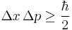
When performing a particular measurement on a quantum state, the result is usually described by a probability distribution, and the form that this distribution takes is completely determined by the quantum state and the observable describing the measurement. These probability distributions are necessary for both mixed states and pure states: It is impossible in quantum mechanics (unlike classical mechanics) to have any state whose properties are all fixed and certain. This is exemplified by the Heisenberg uncertainty principle, and reflects a core difference between classical and quantum physics.
Mathematically, a pure quantum state is typically represented by a vector in a Hilbert space which is a generalization of our more usual three dimensional space. In a Hilbert space the co-ordinates are complex numbers, a complex kind of distance between points is defined and infinite series of numbers are made to converge. In physics, bra-ket notation is often used to denote such vectors. Linear combinations (superpositions) of vectors can describe interference phenomena. Mixed quantum states are described by density matrices.
In a more general mathematical context, quantum states can be understood as positive normalized linear functionals on a C* algebra; see GNS construction.
Contents |
Conceptual description
The state of a physical system
The state of a physical system is a complete description of the parameters of the experiment. To understand this rather abstract notion, it is useful to first explore it in an example from classical mechanics.
Consider an experiment with a (non-quantum) particle of mass  that moves freely, and without friction, in one spatial direction.
We put the particle at initial position  and start the experiment at time
  by pushing the particle with some speed and in some direction. Doing this, we determine the initial momentum
  of the particle. These initial conditions are what characterizes the state
  of the system, formally denoted as
  . We say that we prepare the state of the system by fixing its initial conditions.
At a later time  , we conduct measurements on the particle. The measurements we can perform on this simple system are essentially its position
  at time
  , its momentum
  , and combinations of these. Here and refer to the measurable quantities (observables) of the system as such, not the specific results they produce in a certain run of the experiment.
However, knowing the state of the system, we can compute the value of the observables in the specific state, i.e. the results that our measurements will produce, depending on and . We denote these values as  and
and  . In our simple example, it is well known that the particle moves with constant velocity; therefore,[3]

Now suppose that we start the particle with a random initial position and momentum. (For argument's sake, we may suppose that the particle is pushed away at by some apparatus which is controlled by a random number generator.) The state of the system is now not described by two numbers and , but rather by two probability distributions. The observables and will produce random results now; they become random variables, and their values in a single measurement cannot be predicted. However, if we repeat the experiment sufficiently often, always preparing the same state , we can predict the expectation value of the observables (their statistical mean) in the state . The expectation value of is again denoted by , etc.
These "statistical" states of the system are called mixed states, as opposed to the pure states discussed further below. Abstractly, mixed states arise as a statistical mixture of pure states.
Quantum states
In quantum systems, the conceptual distinction between observables and states persists just as described above. The state of the system is fixed by the way the physicist prepares the experiment (e.g., how the physicist adjusts the particle source). As above, there is a distinction between pure states and mixed states, the latter being statistical mixtures of the former. However, some important differences arise in comparison with classical mechanics.
In quantum theory, even pure states show statistical behaviour. Regardless of how carefully we prepare the state  of the system, measurement results are not repeatable in general, and we must understand the expectation value
  of an observable
  as a statistical mean. It is this mean that is predicted by physical theories.
For any fixed observable , it is generally possible to prepare a pure state  such that has a fixed value in this state: If we repeat the experiment several times, each time measuring , we will always obtain the same measurement result, without any random behaviour. Such pure states are called eigenstates of .
However, it is impossible to prepare a simultaneous eigenstate for all observables. For example, we cannot prepare a state such that both the position measurement and the momentum measurement (at the same time ) produce "sharp" results; at least one of them will exhibit random behaviour.[4] This is the content of the Heisenberg uncertainty relation.
Moreover, in contrast to classical mechanics, it is unavoidable that performing a measurement on the system generally changes its state. More precisely: After measuring an observable , the system will be in an eigenstate of ; thus the state has changed, unless the system was already in that eigenstate. This expresses a kind of logical consistency: If we measure twice in the same run of the experiment, the measurements being directly consecutive in time, then they will produce the same results. This has some strange consequences however:
Consider two observables, and  , where corresponds to a measurement earlier in time than .[5] Suppose that the system is in an eigenstate of . If we measure only , we will not notice statistical behaviour. If we measure first and then in the same run of the experiment, the system will transfer to an eigenstate of after the first measurement, and we will generally notice that the results of are statistical. Thus, quantum mechanical measurements influence one another, and it is important in which order they are performed.
Another feature of quantum states becomes relevant if we consider a physical system that consists of multiple subsystems; for example, an experiment with two particles rather than one. Quantum physics allows for certain states, called entangled states, that show certain statistical correlations between measurements on the two particles which cannot be explained by classical theory. For details, see entanglement. These entangled states lead to experimentally testable properties (Bell's theorem) that allow us to distinguish between quantum theory and alternative classical (non-quantum) models.
Schrödinger picture vs. Heisenberg picture
In the discussion above, we have taken the observables , to be dependent on time, while the state was fixed once at the beginning of the experiment. This approach is called the Heisenberg picture. One can, equivalently, treat the observables as fixed, while the state of the system depends on time; that is known as the Schrödinger picture. Conceptually (and mathematically), both approaches are equivalent; choosing one of them is a matter of convention.
Both viewpoints are used in quantum theory. While non-relativistic quantum mechanics is usually formulated in terms of the Schrödinger picture, the Heisenberg picture is often preferred in a relativistic context, that is, for quantum field theory. Compare with Dirac picture.
Formalism in quantum physics
Pure states as rays in a Hilbert space
Quantum physics is most commonly formulated in terms of linear algebra, as follows. Any given system is identified with some Hilbert space, such that each vector in the Hilbert space (apart from the origin) corresponds to a pure quantum state. In addition, two vectors that differ only by a nonzero complex scalar correspond to the same state (in other words, each pure state is a ray in the Hilbert space; equivalently, a point in the projective Hilbert space.).
Alternatively, many authors choose to only consider normalized vectors (vectors of norm 1) as corresponding to quantum states. In this case, the set of all pure states corresponds to the unit sphere of a Hilbert space, with the proviso that two normalized vectors correspond to the same state if they differ only by a complex scalar of absolute value 1, which is called the phase factor.
Bra-ket notation
Calculations in quantum mechanics make frequent use of linear operators, inner products, dual spaces and Hermitian conjugation. In order to make such calculations more straightforward, and to obviate the need (in some contexts) to fully understand the underlying linear algebra, Paul Dirac invented a notation to describe quantum states, known as bra-ket notation. Although the details of this are beyond the scope of this article (see the article Bra-ket notation), some consequences of this are:
- The variable name used to denote a vector (which corresponds to a pure quantum state) is chosen to be of the form
 (where the "
 " can be replaced by any other symbols, letters, numbers, or even words). This can be contrasted with the usual mathematical notation, where vectors are usually bold, lower-case letters, or letters with arrows on top.
 - Instead of vector, the term ket is used synonymously.
- Each ket is uniquely associated with a so-called bra, denoted
 , which is also said to correspond to the same physical quantum state. Technically, the bra is an element of the dual space, and related to the ket by the Riesz representation theorem.
 - Inner products (also called brackets) are written so as to look like a bra and ket next to each other:
 . (Note that the phrase "bra-ket" is supposed to resemble "bracket".)
Spin, many-body states
It is important to note that in quantum mechanics besides, e.g., the usual position variable  , a discrete variable m exists, corresponding to the value of the z-component of the spin vector. This can be thought of as a kind of intrinsic angular momentum. However, it does not appear at all in classical mechanics and arises from Dirac's relativistic generalization of the theory. As a consequence, the quantum state of a system of N particles is described by a function with four variables per particle, e.g.
 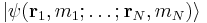 . Here, the variables mν assume values from the set {
 }, where
  (in units of Planck's reduced constant
  ), is either a non-negative integer (0,1,2...; bosons), or semi-integer (1/2,3/2,5/2,...; fermions). Moreover, in the case of identical particles, the above N-particle function must either be symmetrized (in the bosonic case) or anti-symmetrized (in the fermionic case) with respect to the particle numbers.
Electrons are fermions with S = 1/2, photons (quanta of light) are bosons with S = 1.
Apart from the symmetrization or anti-symmetrization, N-particle states can thus simply be obtained by tensor products of one-particle states, to which we return herewith.
Basis states of one-particle systems
As with any vector space, if a basis is chosen for the Hilbert space of a system, then any ket can be expanded as a linear combination of those basis elements. Symbolically, given basis kets  , any ket can be written
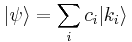
where ci are complex numbers. In physical terms, this is described by saying that has been expressed as a quantum superposition of the states . If the basis kets are chosen to be orthonormal (as is often the case), then  .
.
One property worth noting is that the normalized states are characterized by
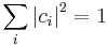
Expansions of this sort play an important role in measurement in quantum mechanics. In particular, if the are eigenstates (with eigenvalues  ) of an observable, and that observable is measured on the normalized state , then the probability that the result of the measurement is ki is |ci|2. (The normalization condition above mandates that the total sum of probabilities is equal to one.)
A particularly important example is the position basis, which is the basis consisting of eigenstates of the observable which corresponds to measuring position. If these eigenstates are nondegenerate (for example, if the system is a single, spinless particle), then any ket is associated with a complex-valued function of three-dimensional space:
 .
.
This function is called the wavefunction corresponding to .
Superposition of pure states
One aspect of quantum states, mentioned above, is that superpositions of them can be formed. If  and
and  are two kets corresponding to quantum states, the ket
is a different quantum state (possibly not normalized). Note that which quantum state it is depends on both the amplitudes and phases (arguments) of  and
and  . In other words, for example, even though and
  (for real θ) correspond to the same physical quantum state, they are not interchangeable, since for example
  and
and  do not (in general) correspond to the same physical state. However, and
  do correspond to the same physical state. This is sometimes described by saying that "global" phase factors are unphysical, but "relative" phase factors are physical and important.
One example of a quantum interference phenomenon that arises from superposition is the double-slit experiment. The photon state is a superposition of two different states, one of which corresponds to the photon having passed through the left slit, and the other corresponding to passage through the right slit. The relative phase of those two states has a value which depends on the distance from each of the two slits. Depending on what that phase is, the interference is constructive at some locations and destructive in others, creating the interference pattern.
Another example of the importance of relative phase in quantum superposition is Rabi oscillations, where the relative phase of two states varies in time due to the Schrödinger equation. The resulting superposition ends up oscillating back and forth between two different states.
Mixed states
A pure quantum state is a state which can be described by a single ket vector, as described above. A mixed quantum state is a statistical ensemble of pure states (see quantum statistical mechanics). Equivalently, a mixed-quantum state on a given quantum system described by a Hilbert space H naturally arises as a pure quantum state (called a purification) on a larger bipartite system H tensor K, the other half of which is inaccessible to the observer.
A mixed state cannot be described as a ket vector. Instead, it is described by its associated density matrix (or density operator), usually denoted . Note that density matrices can describe both mixed and pure states, treating them on the same footing.
The density matrix is defined as
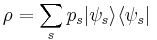
where  is the fraction of the ensemble in each pure state
  Here, one typically uses a one-particle formalism to describe the average behaviour of an N-particle system.
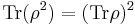
A simple criterion for checking whether a density matrix is describing a pure or mixed state is that the trace of ρ2 is equal to 1 if the state is pure, and less than 1 if the state is mixed.[6] Another, equivalent, criterion is that the von Neumann entropy is 0 for a pure state, and strictly positive for a mixed state.
The rules for measurement in quantum mechanics are particularly simple to state in terms of density matrices. For example, the ensemble average (expectation value) of a measurement corresponding to an observable is given by

where  are eigenkets and eigenvalues, respectively, for the operator , and tr denotes trace. It is important to note that two types of averaging are occurring, one being a quantum average over the basis kets
  of the pure states, and the other being a statistical average with the probabilities of those states.
W.r.t. these different types of averaging, i.e. to distinguish pure and/or mixed states, one often uses the expressions 'coherent' and/or 'incoherent superposition' of quantum states.
Mathematical formulation
For a mathematical discussion on states as functionals, see Gelfand–Naimark–Segal construction. There, the same objects are described in a C*-algebraic context.
See also
- Basic concepts of quantum mechanics
- Excited state
- Introduction to quantum mechanics
- Orthonormal basis
- Probability amplitude
- Quantum harmonic oscillator
- Qubit
- Stationary state
- W state
- Wave function
Notes
- ^ Feynman, Richard P.; Leighton R.B. Sands M. (1965). "4.2". The Feynman Lectures on Physics Vol. 3 Quantum Mechanics. USA: Addison–Wesley Publishing Company. pp. 4-3.
- ^ http://www.quantiki.org/wiki/Bloch_sphere
- ^ In this example, momentum p = velocity, since p = m · velocity, and m = 1. The system of units for this example has been defined such that mass is unitless.
- ^ To avoid misunderstandings: Here we mean that and are measured in the same state, but not in the same run of the experiment.
- ^ For concreteness' sake, you may suppose that
 and
and  in the above example, with
  .
. - ^ Blum, Density matrix theory and applications, page 39. Note that this criterion works when the density matrix is normalized so that the trace of ρ is 1, as it is for the standard definition given in this section. Occasionally a density matrix will be normalized differently, in which case the criterion is
Further reading
The concept of quantum states, in particular the content of the section Formalism in quantum physics above, is covered in most standard textbooks on quantum mechanics.
For a discussion of conceptual aspects and a comparison with classical states, see:
- Isham, Chris J (1995). Lectures on Quantum Theory: Mathematical and Structural Foundations. Imperial College Press. ISBN 978-1860940019.
For a more detailed coverage of mathematical aspects, see:
- Bratteli, Ola; Robinson, Derek W (1987). Operator Algebras and Quantum Statistical Mechanics 1. Springer. ISBN 978-3540170938. 2nd edition. In particular, see Sec. 2.3.
For a discussion of purifications of mixed quantum states, see Chapter 2 of John Preskill's lecture notes for Physics 219 at Caltech.